Getting Started with Geospatial Data in Snowflake

Background

Skip this section if you understand the fundamentals of geospatial data types and spatial reference systems.

Numeric, string, boolean, and other data types have reference systems. Numeric data types follow the decimal number system. String data types adhere to a character set (computationally represented by the hexadecimal system), while boolean data types follow the binary number system, and so on. You can efficiently perform basic manipulations and operations on these data types. You can also run an analysis on top of the data held in these data types. The underlying reference system powers all these operations performed using the data type.

Although geolocation data, at its most basic level, is just a pair of numbers — latitude and longitude — which can be stored in numeric data types, it is hard to perform real-world calculations on those numbers. The decimal number system alone isn’t enough for storing information about a place on Earth. A system analysing geospatial data must know that the two points lie on a specific surface, even to calculate something as simple as the distance between two points. That’s where a spatial reference system comes into the picture.

Now, most databases use two types of reference systems to map these points to a surface. The first assumes that the planet can be represented as a flat surface on a Cartesian or Euclidian plane, giving birth to the GEOMETRY data type. The second assumes that the planet can be modelled as a perfect sphere, making GEOGRAPHY data type the other option.

Using GEOGRAPHY data type makes more sense when calculating distances across the planet’s surface. On the other hand, the GEOMETRY data type is more useful when visualising data on a two-dimensional map of a geographical area. The good thing is that, if your database allows, you can convert one data type to another using standard built-in functions. That’s it on the brief background. Let’s look at how Snowflake deals with geospatial data!

Working with Geospatial Data in Snowflake

In June 2021, Snowflake’s first geospatial data type — GEOGRAPHY— went GA. This May, they’ve also made the GEOMETRY datatype GA will now help geospatial data analysts and engineers have more flexibility in consuming the data through analysis and visualisation. To understand more about geometric representations in Snowflake, read this post on the Snowflake blog.

Ingesting Geospatial Data into Snowflake

Geospatial data can come in all shapes and sizes. The files you source into Snowflake may have a structure that isn’t very different from a CSV file, with the only difference being that the source files will have latitudes and longitudes. If the data is already processed and shaped up as having a geospatial representation, you can expect it to be in a well-known text format, where you can represent a pair of latitude and longitude as a POINT and a group of latitude and longitude pairs as a MULTILINE or a POLYGON.

There are also other standards and formats that Snowflake supports for ingestion, such as GeoJSON. You can look at the complete list here. There’s a difference between WKT/WKB and GeoJSON, which is worth repeating here from the Snowflake documentation —

This goes back to the context I gave you about reference systems. Anyway, the long and short of it is that your geospatial data can be in various formats to be fit for ingestion. For successful ingestion, you must align or transform (using reference system transform functions like ST_TRANSFORM) your Snowflake table structure and data types according to the source data format and reference system.

Geospatial Data Processing in Snowflake

You may have several use cases for processing geospatial data, i.e., calculating proximity, adjacency, and overlap between points, lines, and polygons, among other things. Geospatial data aggregation is one of the most prominent use cases. Like how you calculate total sales, cumulative sales, etc., for an e-commerce business, you may need to aggregate your geospatial data from a point to a multipoint, a linestring, a polygon, and more, for a logistics business.

Here’s a simple example that comes from a free Snowflake marketplace data share that has data about bike stations in Chicago:

CREATE TABLE ANALYTICS.PUBLIC.STATION_INFO_FLATTEN_SOS AS

WITH bike_station_locations AS
(SELECT REPLACE(station_id,'"','') station_id,
        REPLACE(name,'"','') station_name,
        ST_MAKEPOINT(lon, lat) point
   FROM CHICAGO_DIVVY_BIKE_STATION_STATUS.PUBLIC.STATION_INFO_FLATTEN
  LIMIT 5)
  
SELECT ST_COLLECT(point) point
  FROM bike_station_locations;

SELECT * FROM ANALYTICS.PUBLIC.STATION_INFO_FLATTEN_SOS;

The above piece of SQL reads the latitude and longitude values for the bike station location and converts them into a POINT data type. Once that’s done, it uses the ST_COLLECT aggregation function to convert several points to a MULTIPOINT, which sort of works like the LISTAGG function in Oracle or the GROUP_CONCAT function in MySQL. Here’s what the output will look like:

{
  "type": "FeatureCollection",
  "features": [
    {
      "type": "Feature",
      "properties": {},
      "geometry": {
        "coordinates": [
          [
            -87.673688,
            41.871262
          ],
          [
            -87.6601406209,
            41.98974251144
          ],
          [
            -87.5970051479,
            41.81409271048
          ],
          [
            -87.57632374763489,
            41.78091096424803
          ],
          [
            -87.707322,
            41.921525
          ]
        ],
        "type": "MultiPoint"
      }
    }
  ]
}

Now, if you paste this into any GeoJSON visualiser like geojson.io, you can see the points on a map, as shown in the image below:

There’s a lot more to geospatial data processing. I’ll cover that in more detail in an upcoming post.

Geospatial Search with Search Optimisation Service

Most relational databases that support geospatial data also have constructs for geospatial indexing. Snowflake, on the other hand, doesn’t support indexes. Instead, you can use Snowflake’s Search Optimization Service (SOS) to speed up your geospatial search queries. Here’s how you enable search optimisation on a column:

ALTER TABLE ANALYTICS.PUBLIC.STATION_INFO_FLATTEN_SOS 
  ADD SEARCH OPTIMIZATION ON GEO(point);

Like PostgreSQL, which supports search functionality using specific geospatially-indexed functions, Snowflake does that for some supported functions. Currently, geospatial search optimisation only works for columns with GEOGRAPHY data type. GEOMETRY data type is not supported yet.

Snowflake’s Search Optimization Service helps speed up point look-up queries that answer questions like:

• Whether a geospatial object is fully contained within another geospatial object — a state within a country, a water body within a county, etc., using the ST_WITHIN geospatial function.
• Whether two geospatial objects share any common portion — this turns out to be extremely useful and essential in mapping houses, localities, and communities using the ST_INTERSECTS geospatial function.

This service works better if the data you seek is clustered together. If you don’t already have a geographical distribution column, you can use the ST_GEOHASH function to leverage the proximity grouping method that a geohash employs.

Spatial Partitioning and Indexing with H3

While the Search Optimisation Service enables point look-up queries, many more use cases require a space partitioning system as a discrete global grid. These use cases revolve mostly around location-based aggregation of moving vehicles, IoT devices, traffic lights, and other objects.

Although H3 (Hexagonal Hierarchical Geospatial Indexing System) is more popularly known as an indexing system, it aligns more with partitioning data, i.e., H3 partitions data like a range-based or a key-based partition scheme partitions your data in a relational database. The key difference here is that your partitions are hexagonal boundaries, which have benefits you can read about in the following blog — Why We Use H3.

A quick note on Hexagons — and why they’re better to map to a sphere.

When you want to map the Earth, you want to devise the most efficient way of spatially partitioning it into blocks or sections that don’t leave any space uncovered. This can be achieved by creating a tessellation, a tiling, of polygons, which can either be triangles, squares, or hexagons. These are the only three shapes that can fill a plane or a spherical surface without leaving a gap. A hexagon is the most complex polygon that can fill a plane, which makes it the most accurate when mapping to a spherical-ish surface because of the curvature.

Read the following piece for more info on Hexagonal grids:

Fishnets and Honeycomb: Square vs. Hexagonal Spatial Grids | Matt Strimas-Mackey
Exploring the benefits of hexagonal grids relative to square grids for spatial sampling and analysis, and generating…strimas.com

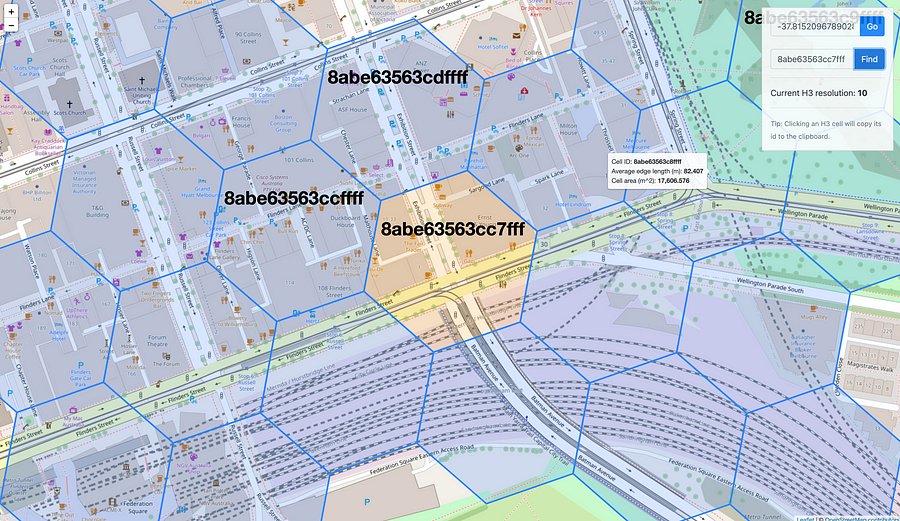
The value of an H3 index is subjective; it depends on two fixed values and one variable value, i.e., latitude, longitude, and the H3 index resolution. When you pass these three things to a function that calculates the H3 value, you uniquely identify a hexagon on the discrete global grid of hexagons. 

Using the values derived from the H3 spatial partitioning system, you can map grid hexagons ranging from approximately one m² to about 4.3 million km², represented with number of hexagons ranging from 569.7 trillion to 122, with resolutions ranging from 15 to 0.

Here’s the grid at resolution 10 with the highlighted hexagon where our Melbourne office is located.

Working with geospatial data, you’ll figure out that the visualisation aspect only comes at the end of the pipeline. Before that, it’s going to be, more or less, the same kind of data processing that gets done with any other form of data. Here’s a quick peek into how H3 values are created using latitude and longitude values at two different resolutions (for two different levels of aggregation)

WITH bike_station_locations AS
(SELECT REPLACE(station_id,'"','') station_id,
        REPLACE(name,'"','') station_name,
        ST_MAKEPOINT(lon, lat) point,
        H3_POINT_TO_CELL(ST_MAKEPOINT(lon, lat),12) h3_index_12,
        H3_POINT_TO_CELL(ST_MAKEPOINT(lon, lat),10) h3_index_10
   FROM CHICAGO_DIVVY_BIKE_STATION_STATUS.PUBLIC.STATION_INFO_FLATTEN
  LIMIT 10)
  
SELECT * 
  FROM bike_station_locations;

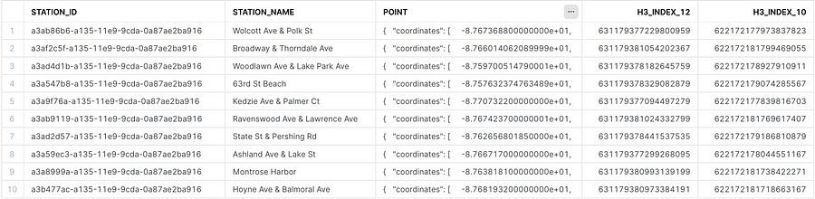
Here’s what the output of this query would look like:

The H3 spatial partitioning system not only helps address the problem of spatial data optimisation but also solves many practical problems, like identifying taxi supply and demand clusters, pinpointing accident-prone areas, and many more.

Snowflake’s geospatial capabilities are well-placed to solve any geospatial ingestion, processing, analysis, and visualisation problem that might come your way. As described in the article, Snowflake extensively supports geospatial data types, specialised indexing, partitioning systems, and more. While this was an introduction to the geospatial capabilities within Snowflake, in a couple of upcoming blogs, I’ll cover a step-by-step approach to ingesting, processing, optimising, converting, and visualising spatial data and how Snowflake handles the visualisation aspect of geospatial data with Streamlit. Meanwhile, you can check out this blog on Streamlit’s website, which discusses exactly that.

Further Reading

• Migrating Spatial Data from PostgreSQL to Snowflake
• Geospatial Functions in Snowflake
• Cell Counts and Resolutions in H3 Indexing
• H3 Indexes and PostGIS
• Snowflake Quickstart — Getting Started with Geospatial
• The Defence Context, Geospatial Standards for Data Science — Dr Paul. Cripps
• The Miraculous Space Efficiency of Honeycomb
• Hexagons are the Bestagons, and Hexagons are NotSoGreatAgons

Credits

Thanks to Matt Dudley and Sagar Kulkarni for generously taking time out and providing feedback on this blog.