A brief guide to methods for creating a global grid system for geospatial indexing and partitioning

ll deterministic data processing is fundamentally based on searching and sorting. To process data efficiently, one needs to search and sort it by discarding all the data they don’t need — that’s what indexes and partitions are for. The details of how indexes and partitions are implemented are usually abstracted away from end users, but different types of indexes and partitions work better with different underlying data types.

Relational databases and data warehouse platforms support indexing types like B-tree, B+ tree, GiST, SP-GiST, and Hash. Some work better for point lookup queries on numbers and short text fields, while others work better for full-text searches, and so on. When it comes to geospatial data, one of the popular index types is the R-tree, about which the PostgreSQL documentation says the following:

R-Trees break up data into rectangles, and sub-rectangles, and sub-sub rectangles, etc. It is a self-tuning index structure that automatically handles variable data density, differing amounts of object overlap, and object size.

This has many variations in kd-tree, Quadtree, Octree, and other indexing methods that help you index geospatial data. These indexing methods are included in the database’s low-level implementation, meaning that adding, removing, or changing the data can lead to expensive tree rebalancing and index rebuilding. This can both increase the computing cost and affect the performance of ongoing queries. Because of this limitation, various data processing systems have developed pluggable geospatial indexing and partitioning systems that decouple indexing from core database operations. These are based on the idea that the surface of the Earth can be represented as a grid system. From Uber’s engineering blog:

A global grid system usually requires at least two things: a map projection and a grid laid on top of the map. A map projection is needed for going from a three-dimensional location on Earth to a two dimensional point on a map. A grid is then overlaid on the map, forming a global grid system.

In this article, I will outline some of these systems and their background, focusing on Google’s S2, Uber’s H3, and Bing Maps’ Quadbin indexing methods. But before we get started, let’s take a quick look at how indexing and partitioning work in geospatial data.

Indexing vs. Partitioning in Grid Systems

In the traditional database sense, indexing means creating a pointer table based on specific columns ordered a certain way. Partitioning, in the same context, is usually the physical separation of files under the same logical construct of a table.

While many types of indexing methodologies are available in the geospatial world, which we will discuss in a while, it is important to note that they are not really indexing techniques. Instead, they’re partitioning techniques.

Why do I say this? Indexes usually help you order data in a certain way to facilitate faster retrieval, while partitions help you segregate data for the same purpose. When it comes to geospatial data, what we’re doing with popular geospatial indexing techniques like S2, H3, and Quadbin is partitioning, not indexing.

That’s why Uber H3’s documentation says that H3 is a Hexagonal Hierarchical Spatial Index, which “enables users to partition the globe into hexagons for more accurate analysis.” Let’s understand some of the grid system partitioning methods now.

Grid System Indexing and Partitioning Methods

While many indexing (read partitioning) methods exist, four stand out because of their wide adoption and support in many data processing and visualization systems. Three of these four, S2, H3, and Quadbin, came from three large companies trying to solve maps for navigation, while Geohash was created by Canonical’s CTO, Gustavo Niemeyer.

Geohash

It’s the oldest of the four methods we discussed. Geohash’s author made it public in 2008. It is based on the equirectangular projection, which was invented thousands of years ago. It has its shortcomings, as do the others that we will discuss. After all, we are trying to map an irregularly shaped ellipsoid (our beautiful planet) to a perfect rectangle. What could go wrong? Indulge yourself in watching this short video that explains the trouble with projections

Nevertheless, it is one of the most popular methods for implementing proximity searches. It is a system for encoding location in strings, not numbers while creating a hierarchical quadtree grid system. It is used for place identification, but a more popular, human-readable sort of hash would be what3words, a service that converts any lat long pair to a square of area 3m² identifiable with three words like ///candy.wire.dull. That’s our Versent Melbourne office, by the way.

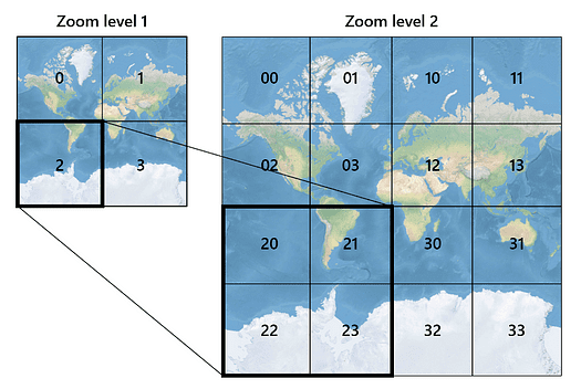
Geohash can go to an arbitrary number of levels. When you zoom in, you break the squares into four, forcing them to be arranged into a tree that will later be used for search and traversal. This is where a Z-order curve comes in. It orders these smaller squares, automatically enabling you to perform a breadth-first search on your whole tree.

Interestingly, Z-order curves are also used to reorganize data on disk to speed up queries. This feature is natively implemented in the Delta Lake file format. The Databricks documentation says the following:

Z-ordering is a technique to colocate related information in the same set of files. This co-locality is automatically used by Delta Lake on Databricks data-skipping algorithms. This behavior dramatically reduces the amount of data that Delta Lake on Databricks needs to read.

The Cloudera blog also talks about using Z-order curves to speed up queries, and so do Apache Hudi, AWS DynamoDB, and Aurora MySQL, among others

However, using Geohash (and Z-order curves to traverse) doesn’t come without challenges, mainly because of the choice of projection and the grid shape used. One major drawback is significant variations in squares at different latitudes. There are also limitations around inaccuracies in proximity searches closer to the boundary of the geohash square, i.e., points closer to the geohash boundary will end up having quite different hashes, hence unrecognizable.

Google’s S2

Geospatial processing can be compute-intensive. To mitigate this issue, Google’s open-source indexing library, S2, assumes Earth as a perfect mathematical sphere, making specific geospatial processing easier and less expensive.

Announcing the S2 Library: Geometry on the Sphere

S2 is the only one of the three methods we’re discussing that represents the data in a hierarchy of quadrilaterals represented on a three-dimensional sphere. Because of this, S2 shows less distortion towards the extremes of the northern and southern hemispheres.

S2 offers a wide range of shapes and sizes that you can use to partition your grid using spherical caps or discs, latitude-longitude rectangles, polylines, and polygons. This makes S2 a good choice for implementing proximity-based searches, simplifying geographies, and quick lookups.

Note that the percentage of area signifies the accuracy of a partitioning method it can successfully represent under all its partitions combined. S2 uses a function based on the continuous and space-filling Hilbert curve that visits every point in a unit square to break a sphere into smaller chunks; it’s how you traverse (and search) the grid on your map.

Spatial Index: Space-Filling Curves

This was worth mentioning because grid traversal, although with slightly different techniques, reappears when discussing H3 and Quadbin. For a deeper look, read the following:

• Grid System Spatial Analysis in BigQuery
• Google’s S2, geometry on the sphere, cells, and Hilbert curve

Google’s S2 suffers, however, from the same drawbacks as Geohash. The grid cells aren’t equidistant from all their neighbours, which makes things difficult in many use cases. At least there’s a guarantee that a data point will always land in only one grid cell, unlike Uber’s H3, which can land in multiple cells, which we’ll come to a bit later. S2, in many ways, is better than Geohash but doesn’t have the portability, interoperability, and widespread support of Geohash, which is why it might be a hard sell.

Quadbin

Bing Maps launched in the same year as Google Maps, i.e., 2005, but took a different approach to mapping the globe when it used Quadtrees (conceptually quite similar to geohashes). Bing Maps’ Quadtree goes up to 23 levels. This implementation by Bing Maps is called Quadkey.

Quadbin is a hierarchical index based on Quadkey. It stores grid cell values in a 64-bit number and goes a bit further concerning the level of detail to 27 levels, which can point to areas less than 1m². Bing Maps uses the Mercator projection, which comes with its challenges. While Bing Maps will be deprecated sometime in 2025, Azure Maps will continue to use the Spherical Mercator projection coordinate system.

Uber’s H3

While the rest of the systems we’ve discussed use rectangles and squares to create a mappable global grid, H3 uses hexagons, assuming the globe to be a regular icosahedron instead of a perfect sphere. This differs from Geohash (which uses an equirectangular projection), S2 (which uses a stereographic projection), and Quadbin (which uses a Mercator projection). The original blog post announcing the open-sourcing of H3 says the following about this choice:

This projects from Earth as a sphere to an icosahedron, a twenty-sided platonic solid. An icosahedron-based map projection results in twenty separate two-dimensional planes rather than a single plane. The icosahedron can be unfolded in many ways, producing a two-dimensional map each time. H3, however, does not unfold the icosahedron to build its grid system, and instead lays its grid out on the icosahedron faces themselves, forming a geodesic discrete global grid system.

I’ve already discussed H3 in another piece covering geospatial data ingestion, indexing, and analysis in Snowflake. I also discuss why hexagons have the edge when calculating grid distances, proximity searches, and navigation.

Getting Started with Geospatial Data in Snowflake

Ben Feifke’s blog post about these systems has a section at the end that compares these three indexing/partitioning systems and discusses when to use which one.

Support for Geohash, S2, H3, and Quadbin

These indexing and partitioning systems are available in most databases and data warehouse systems. They can be used independently as they can be decoupled from the database’s core indexing implementation. For example, Foursqaure’s layer library offers H3, S2, and Hexbin layers that can be used in analytical calculations or as overlays on top of existing geospatial visualizations.

The support for different grid systems, especially H3 and Geohash, is exceptionally promising across the data ecosystem. PostgreSQL, Snowflake, Databricks, ClickHouse, and even newer databases like DuckDB have extensions or built-in libraries. This means you can use the indexing and partitioning system that suits your use case.

Conclusion

My experience working with geospatial indexing and partitioning systems has been with PostgreSQL with PostGIS (the OG, I’d say), Redshift, and MySQL, among others. Recently, though, I’ve been spending quite a bit of time exploring Snowflake for geospatial data, and it’s becoming more promising by the day. Check out the end of June 2024 update regarding new H3 functions to know more.

I hope this overview of geospatial indexing and partitioning systems has been useful to you. I’m working on my next post in this series exploring geospatial data, which will examine an actual use case using one of the database systems mentioned above.

Thanks to Kroum Kluctchkov, Dima Marr, and Haymang Ahuja for providing feedback on this blog post.